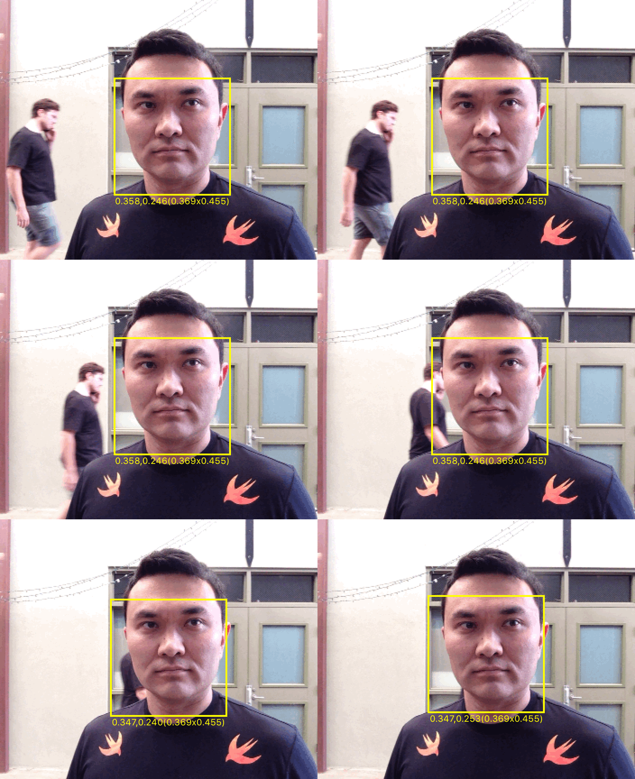
Apple has been using machine learning in their products for a long time: Siri answers our questions and entertains us, iPhoto recognizes faces in our photos, Mail app detects spam messages.
As app developers, we have access to some capabilities exposed by Apple’s APIs such as face detection, and starting with iOS 10, we’ll gain a high-level API for speech recognition and SiriKit.
Sometimes we may want to go beyond the narrow confines of the APIs that are built into the platform and create something unique. Many times, we roll our own machine learning capabilities, using one of a number of off-the-shelf libraries or building directly on top of fast computation capabilities of Accelerate or Metal.
For example, my colleagues built an entry system for our office that uses an iPad to detect a face, then posts a gif in Slack and allows users to unlock the door using a custom command.

But now we have first-party support for neural networks: at WWDC 2016, Apple introduced not one, but two neural network APIs, called Basic Neural Network Subroutines (BNNS) and Convolutional Neural Networks (CNN).
Machine Learning and Neural Networks
AI pioneer Arthur Samuel defined machine learning as a “field of study that gives computers the ability to learn without being explicitly programmed.” Machine learning systems are frequently used to make sense of the data that can’t easily be described using traditional models.
For example, we can easily write a program that calculates the square footage (area) of the house, given the dimensions and shapes of all its rooms and other spaces, but calculating the value of the house is not something we can put in a formula. A machine learning system, on the other hand, is well suited for such problems. By supplying the known real-world data to the system, such as the market value, size of the house, number of bedrooms, etc., we can train it to be able to predict the price.
A neural network is one of the most common models to building machine learning system. While the mathematical underpinnings of neural networks have been developed over half a century ago in the 1940s, parallel computing made them more feasible in the 1980s and the interest in deep learning sparked a resurgence of neural networks in the 2000s.
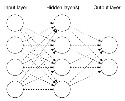
A neural network is constructed of a number of layers, each of which consists of one or more nodes. The simplest neural network has three layers: input, hidden and output. The input layer nodes may represent individual pixels in an image or some other parameters. The output layer nodes are often the results of the classification, such as “dog” or “cat”, if we are trying to automatically detect the contents of a photo. The hidden layer nodes are configured to perform an operation on the inputs or apply the activation function.

Types of Layers
Three common types of layers are pooling, convolution and fully connected.
A pooling layer aggregates the data, reducing its size, typically by using the maximum or average value of its inputs. A series of convolution and pooling layers can be stringed together to gradually distill a photo into a collection of increasingly higher-level features.
A convolution layer transforms an image by applying a convolution matrix to each pixel of the image. If you’ve used Pixelmator or Photoshop filters, you’ve most likely used a convolution matrix. A convolution matrix is typically a 3×3 or 5×5 matrix that is applied to the input image pixels in order to calculate the new pixel values in the output image. To get the value of the output pixel, we would multiply the values of the pixels in the original image and calculate the average.
For example, this convolution matrix would blur the image:
Whereas this one would sharpen the image:
The neural network’s convolution layer uses the convolution matrix to process the input and generate the data for the next layer, for example, to extract new features in an image, such as edges.
A fully connected layer can be thought of as a convolution layer where the filter has the same size as the original image. In other words, you can think of the fully connected layer as a function that assigns weights to individual pixels, averages the result, and gives a single output value.
Training and Inference
Each layer needs to be configured with appropriate parameters. For example, the convolution layer needs information about the input and output images (dimensions, number of channels, etc.), as well as convolution layer parameters (kernel size, matrix, etc.). The fully connected layer is defined by the input and output vectors, activation function, and weights.
To obtain these parameters, the neural network has to be trained. This is accomplished by passing the inputs through the neural network, determining the output, measuring the error (i.e., how far off the actual result was from the predicted result), and adjusting the weights via backpropagation. Training a neural network may require hundreds, thousands, or even millions of examples.
At the moment, Apple’s new machine learning APIs can be used for building neural networks that only do inference, but not training. Good thing that Big Nerd Ranch does.
Accelerate: BNNS
The first new API is part of the Accelerate framework and is called BNNS, which stands for Basic Neural Network Subroutines. BNNS complements the BLAS (Basic Linear Algebra Subroutines), which was used in some third-party machine learning applications.
BNNS defines layers in the BNNSFilter class. Accelerate supports three types of layers: convolution layer (created by the BNNSFilterCreateConvolutionLayer function), fully connected layer (BNNSFilterCreateFullyConnectedLayer), and pooling layer (BNNSFilterCreatePoolingLayer).
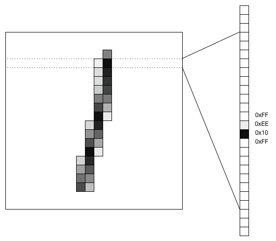
The MNIST database is a well-known data set containing tens of thousands of hand-written digits that were scanned and resized to fit a 20 by 20 pixel image.
One approach to processing image data is to convert an image into a vector and pass it through a fully connected layer. For the MNIST data, a single 20×20 image would become a vector of 400 values. Here’s how a hand-written digit “1” would get converted to a vector:

Below is sample code for configuring a fully connected layer that takes a vector of size 400 as an input, uses the sigmoid activation function and outputs a vector of size 25:
    // input layer descriptor
    BNNSVectorDescriptor i_desc = {
        .size = 400,
        .data_type = BNNSDataTypeFloat32,
        .data_scale = 0,
        .data_bias = 0,
    };

    // hidden layer descriptor
    BNNSVectorDescriptor h_desc = {
        .size = 25,
        .data_type = BNNSDataTypeFloat32,
        .data_scale = 0,
        .data_bias = 0,
    };

    // activation function
    BNNSActivation activation = {
        .function = BNNSActivationFunctionSigmoid,
        .alpha = 0,
        .beta = 0,
    };

    BNNSFullyConnectedLayerParameters in_layer_params = {
        .in_size = i_desc.size,
        .out_size = h_desc.size,
        .activation = activation,
        .weights.data = theta1,
        .weights.data_type = BNNSDataTypeFloat32,
        .bias.data_type = BNNSDataTypeFloat32,
    };

    // Common filter parameters
    BNNSFilterParameters filter_params = {
        .version = BNNSAPIVersion_1_0;   // API version is mandatory
    };

    // Create a new fully connected layer filter (ih = input-to-hidden)
    BNNSFilter ih_filter = BNNSFilterCreateFullyConnectedLayer(&i_desc, &h_desc, &in_layer_params, &filter_params);

    float * i_stack = bir; // (float *)calloc(i_desc.size, sizeof(float));
    float * h_stack = (float *)calloc(h_desc.size, sizeof(float));
    float * o_stack = (float *)calloc(o_desc.size, sizeof(float));

    int ih_status = BNNSFilterApply(ih_filter, i_stack, h_stack);
Does it get any more metal than this? As a matter of fact, it does, because the second neural network API is part of Metal Performance Shaders (MPS) framework. While Accelerate is the framework for performing fast computing on the CPU, Metal pushes the GPU to its limit. Metal’s flavor is called CNN, the Convolution Neural Network.
MPS comes with a similar set of APIs. Creating a convolution layer requires use of MPSCNNConvolutionDescriptor and MPSCNNConvolution functions. For a pooling layer, MPSCNNPoolingMax would supply the parameters. A fully connected layer is created by the MPSCNNFullyConnected function.
The activation functions are defined by subclasses of MPSCNNNeuron: MPSCNNNeuronLinear, MPSCNNNeuronReLU, MPSCNNNeuronSigmoid, MPSCNNNeuronTanH, MPSCNNNeuronAbsolute.
BNNS and CNN compared
This table presents the list of activation functions in Accelerate and Metal:
| Accelerate/BNNS |
Metal Performance Shaders/CNN |
| BNNSActivationFunctionIdentity |
|
| BNNSActivationFunctionRectifiedLinear |
MPSCNNNeuronReLU |
| |
MPSCNNNeuronLinear |
| BNNSActivationFunctionLeakyRectifiedLinear |
|
| BNNSActivationFunctionSigmoid |
MPSCNNNeuronSigmoid |
| BNNSActivationFunctionTanh |
MPSCNNNeuronTanH |
| BNNSActivationFunctionScaledTanh |
|
| BNNSActivationFunctionAbs |
MPSCNNNeuronAbsolute |
Pooling functions:
| Accelerate/BNNS |
Metal Performance Shaders/CNN |
| BNNSPoolingFunctionMax |
MPSCNNPoolingMax |
| BNNSPoolingFunctionAverage |
MPSCNNPoolingAverage |
Accelerate and Metal provide a very similar set of functionality for neural networks, so the choice of one or the other will depend on each application. While GPUs are typically preferred for the kinds of computations required in machine learning, data locality may cause the Metal CNN to perform poorer than the Accelerate BNNS version. If the neural network operates on images that have been loaded into the GPU, for example, using MPSImage and the new MPSTemporaryImage, Metal is the clear winner.
Want more info on machine learning? Check out this post on getting started with Core ML, a new framework announced at WWDC 2017.


