The post Why foray into machine learning? appeared first on Big Nerd Ranch.
]]>Big Nerd Ranch has made our name in Mac and mobile. We were the first to have a comprehensive method for teaching Mac programming, iOS programming, and Android programming. Our deep knowledge of these technologies, forged through real client experience, coupled with our deep empathy for students and how they learn, has allowed us to help thousands of individuals and hundreds of companies to build their own native mobile applications. We think of ourselves as a friendly guide, helping our students solve problems one-by-one until they eventually develop a deep and comprehensive understanding of how to build a quality application that will hold up over the long term.
The transition to mobile involved a massive shift in capabilities and mindset. Designing and building for the small screen was new to most, so they needed comprehensive and high-qualiity training to capitalize on the opportunities afforded by this new technology. Big Nerd Ranch was able to train digital staff from across the spectrum, showing them what was possible with this new technology and giving them the confidence to build and explore more.
It worked. We have been able to train and guide digital companies that have gone on to become household names: Nextdoor, Facebook, just to name a couple. These companies, and many like them, leveraged our training to catapult themselves into the mobile and digital age, often seeing incredible results from their efforts.
Still mobile – now machine learning
Mobile continues to be a critical component of every company’s digital strategy, and we continue to dedicate ourselves to enabling individuals, teams, and organizations in the mobile space. Over the past few years, we have seen that machine learning and artificial intelligence have become the latest frontiers in the digital landscape. Aside from all of the recent news about AI and ML, we know they are prevalent because our clients have increasingly looked to incorporate these technologies into their digital products. Like mobile technologies, machine learning offers an entirely new set of tools with which designers, product owners, and engineers can bring their ideas to life. And like mobile technologies, there is currently a wide gulf between the promise the technology holds and the knowledge and skills organizations have to capitalize on that promise.
That’s why we created our Explore Machine Learning course. We want to serve a similar role as we have in the mobile space: acting as the friendly guide helping individuals, teams, and organizations to unlock the potential of machine learning for their digital products and services. We felt that we were uniquely positioned to guide teams and organizations into this new world, having done so with the last major technology wave and because we continue to keep up with new and emerging technologies.
Machine Learning – what you will learn
We built the course with three key things in mind: 1) demistify machine learning by defining key terms and explaining how the pieces fit together 2) enable students to determine if machine learning is an appropriate tool for their problem space 3) empower students to understand how to integrate machine learning solutions into their current projects. We wanted to show teams the range of machine learning approaches: some can be implemented relatively easily, others not so much. We know that there are entire advanced degree programs on this topic, so our focus was not on replacing them. We wanted to give students an accessible entry point to the technology and as we always have, show them what’s possible, and give them the confidence to explore more.
So whether you are a product owner or software engineer, a business leader or a designer, this course was designed to demistify the world of machine learning and help you understand what it really takes to implement a machine learning solution. Here’s what you’ll learn:
- The basics of machine learning and begin to understand what’s important in the world of machine learning. You learn what the ‘magic’ of machine learning is so that you can converse fluently about it.
- How to leverage existing machine learning solutions to solve your own product and development problems. Explore platform APIs, frameworks, and pre-built models to solve common machine learning problems.
- About data collection and key factors to consider, and gain experience collecting and manually labeling data.
- How to get started on a machine learning project. After seeing the fundamental building blocks and learning how to leverage existing systems, get a taste of what it’s like to build your own simple model.
If these applications of ML pique your interest, we would love to help you, your team, or your organization level up on machine learning. Reach out to us if you are interested in attending a bootcamp or want to set up a course for your team. Happy coding!
The post Why foray into machine learning? appeared first on Big Nerd Ranch.
]]>The post An intro to Machine Learning in iOS with Swift, and Playgrounds appeared first on Big Nerd Ranch.
]]>But wait, why do we even need machine learning and how can it help us? Machine learning allows you to take large data sets and apply complex mathematical calculations over and over, faster and faster.
Apple has made the entry-level for machine learning quite accessible and wrapped it up in an all-in-one package. Swift, Xcode, and Playgrounds are all the tools you’re going to need to train a model, then implement it into a project. If you haven’t already, you’ll want to download Xcode. Now, let’s jump right in.
A note before we begin. This tutorial will be done in Playgrounds to help understand the code behind training models, however, CreateML is a great alternative to training models with no machine learning experience. It allows you to view model creation workflows in real-time.
Training a Model
One of the first things you’re going to need before opening Xcode is a dataset. What’s a dataset you say? It’s simple, a dataset is a collection of data, such as movie reviews, locations of dog parks, or images of flowers. For your purposes, we’re going to be using a file named appStore_description.csv to train your model. There are a handful of resources to find datasets, but we’re using kaggle.com, which is a list of AppStore app descriptions and the app names. We’ll use this text to help predict an app for the user based on their text input. Our model will be a TextClassifier, which learns to associate labels with features of our input text. This could come in the form of a sentence, paragraph, or a whole document.
- Download the dataset here.
- Your dataset may have a column named
track_name, you can open thecsvfile and rename that column toapp_nameso it’s consistent with this example.
Now that you have your dataset you can open Xcode 🙌.
- First, create a new
Playgroundusing themacOStemplate and chooseBlank. We usemacOSbecause theCreateMLframework is not available oniOS. - Delete all the code in the Playground and import
FoundationandCreateML. - Add the dataset to the Playground’s
Resourcesfolder.
Here is what your Playground will look like and what is going on inside it:
import Foundation
import CreateML

//: Create a URL path to your dataset and load it into a new MLDataTable
let filePath = Bundle.main.url(forResource: "appStore_description", withExtension: "csv")
let data = try MLDataTable(contentsOf: filePath)
//: Create two mutually exclusive, randomly divided subsets of the data table
//: The trainingData will hold the larger portion of rows
let (trainingData, testData) = data.randomSplit(by: 0.8)
//: Create your TextClassifier model using the trainingData
//: This is where the `training` happens and will take a few minutes
let model = try MLTextClassifier(trainingData: trainingData, textColumn: "app_desc", labelColumn: "app_name")
//: Test the performance of the model before saving it. See an example of the error report below
let metrics = model.evaluation(on: testData, textColumn: "app_desc", labelColumn: "app_name")
print(metrics.classificationError)

let modelPath = URL(fileURLWithPath: "/Users/joshuawalsh/Desktop/AppReviewClassifier.mlmodel")
try model.write(to: modelPath)
Once you have this in your Playground, manually run it to execute training and saving the model. This may take a few minutes. Something to note is that our original csv dataset file is 11.5 MB and our training and test models are both 1.3 MB. While these are relatively small datasets, you can see that training our model drastically reduces the file size 👍.
Example Error Report
Printing the metrics is optional when creating your model, but it’s good practice to do this before saving. You’ll get an output something like this:
Columns:
    actual_count    integer
    class    string
    missed_predicting_this    integer
    precision    float
    predicted_correctly    integer
    predicted_this_incorrectly    integer
    recall    float
Rows: 1569
Data:
+----------------+----------------+------------------------+----------------+---------------------+
| actual_count   | class          | missed_predicting_this | precision      | predicted_correctly |
+----------------+----------------+------------------------+----------------+---------------------+
| 1              | "HOOK"         | 1                      | nan            | 0                   |
| 1              | ( OFFTIME ) ...| 0                      | nan            | 1                   |
| 1              | *Solitaire*    | 0                      | nan            | 1                   |
| 1              | 1+2=3          | 0                      | nan            | 1                   |
| 1              | 10 Pin Shuff...| 0                      | nan            | 1                   |
| 1              | 10 – �..       | 0                      | nan            | 1                   |
| 1              | 100 Balls      | 0                      | nan            | 1                   |
| 1              | 1010!          | 0                      | nan            | 1                   |
| 1              | 12 Minute At...| 0                      | nan            | 1                   |
| 1              | 20 Minutes.f...| 0                      | nan            | 1                   |
+----------------+----------------+------------------------+----------------+---------------------+
+----------------------------+----------------+
| predicted_this_incorrectly | recall         |
+----------------------------+----------------+
| 0                          | 0              |
| 0                          | 0              |
| 0                          | 0              |
| 0                          | 0              |
| 0                          | 0              |
| 0                          | 0              |
| 0                          | 0              |
| 0                          | 0              |
| 0                          | 0              |
| 0                          | 0              |
+----------------------------+----------------+
[1569 rows x 7 columns]
Adding the model to your app
Now that you have your model trained and saved somewhere on your computer, you can create a new iOS project.
- Let’s make it a single view app and we’ll call it
AppPredictor, and use Storyboards. - Find where you saved your model, and drag that file into your project in Xcode.

- In
ViewController.swiftimportUIKit,NaturalLanguageandCoreML.
import UIKit
import NaturalLanguage
import CoreML
Using your custom text classifier
For simplicity’s sake, your UI will have 3 elements. A text field, a label, and a button. We’re going for functionality here, but feel free to update your designs however you see fit. Next, add the text field, label, and button to your view controller in the storyboard. The text field and label will be IBOutlets, and your button will be an IBAction.
@IBOutlet weak var textField: UITextField!
@IBOutlet weak var appNameLabel: UILabel!

@IBAction func predictApp(_ sender: Any) {

}
Now add a reference to your classifier like so:
private lazy var reviewClassifier: NLModel? = {
    // Create a custom model trained to classify or tag natural language text.
    // NL stands for Natual Language
    let model = try? NLModel(mlModel: AppReviewClassifier().model)
    return model
}()
Let’s then create a function that takes in a string, and returns a string based on the user’s input.
private func predict(_ text: String) -> String? {
    reviewClassifier?.predictedLabel(for: text)
}
Back in predictApp, add the predict function and pass the text fields text in the argument.
appNameLabel.text = predict(textField.text ?? "")
Build and run your app and let’s see what you get. Describe an app that you can’t quite remember the name of, but you know what it does. I described two similar types of apps but got different results 👍.
  |
  |
Conclusion
Machine learning isn’t all that scary or complicated once you break it down into digestible chunks. Finding the right dataset can often be the biggest hurdle. Now that you have the basics down you should explore some of the other classifier types, and train different models.
The post An intro to Machine Learning in iOS with Swift, and Playgrounds appeared first on Big Nerd Ranch.
]]>The post Validating Proof of Concepts before Data Collection appeared first on Big Nerd Ranch.
]]>This is not to say your team doesn’t think it will be worth it. However, when moonshot ideas come up, you have to consider things like if the data is available, and whether the problem is even solvable with this kind of data or model.
This problem of product validation without real data is demonstrated in a recent project that the team at BNR worked on. We were asked to find small objects on a label using compute vision. The catch was the objects are very small and the label itself less than an inch square. We were also going into the project with no data previously collected.
This posed an interesting problem for us. In the everyday world of object detection, you are normally looking for large objects, like people or cars. These very complex multi-pixel objects, when passed into a neural network and compressed, create very unique signatures. To make things more difficult, all the training data was collected at the start of the project.
Before contracts were signed our machine learning team wanted to make sure we could in fact build brilliance and deliver what the client was asking for. Normally we would look up research papers and form a game plan on what models might perform well and what preprocessing we might need to build. However, small objects a few pixels wide are not covered by really any research papers.
So we decided to generate our own synthetic dataset aimed at being harder conditioned than we were expecting with the goal of seeing if we could find the bounds to a successful model. But, we had a big limitation to our research at this point as there was no signed contract and we needed to make the data and train a model fast so we can feel good about green-lighting the project.
Building the generator
The goal was to build a small image with a barcode in the middle. We were going to try and find how small we can make this while still finding good data. So we used a Datamax barcode as they are the smaller of the 2d barcodes. We’ll also lay down flecks and record the location of all of them. Below is a result from our code.

We only need a few tools to make these images. The main one for this task is the pylibdmtx library. This tool allows users to generate Datamax barcodes easily. The pillow library, or PIL, is used to create and manipulate images in python. The last important library is pandas that allowed us to create our dataset on the object location.
The settings of our label are below. Most notably our label will be 160px, contain 40 objects, and we will create a total of 4000 images.
During the process, we randomly pick the location for objects. The size of the objects are fixed at 2px squared and we assigned them one of two colors. Using pandas we added each of the bounding boxes to a data frame for training.
What data to add to the bounding box depends on the model you end up using. A Faster-RCNN model, for instance, wants xmin, ymin, xmax, ymax for the bounding box variables. A YOLO model requires x, y, width, height where x and y are the center of the object. Below we have an example of our output.
,image,name,xMin,yMin,xMax,yMax
0,0.png,BARCODE,145,145,655,655
1,0.png,GOLD_FLAKE,346,161,358,173
2,0.png,GOLD_FLAKE,117,734,129,746
Building a model
When picking out a model for prototyping we weren’t worried about platform or deployment issues. We really wanted to know if a generic object detection algorithm could be trained to solve this problem.
One item we took into consideration is cost. Normally we would use a cloud platform to get extra power as object detection problems can take a very long time to reach convergence. But we couldn’t run up compute cost for the prototype so trained locally on our laptop. Luckily we have access to an eGPU with a Vega GPU.
With our hardware selected we needed a tool that allowed us to quickly train an object detector with an AMD gpu on macOS. As of this writing, we have access to Create ML, Turi Create, and PlaidML as tools on macOS that give us access to the eGPU for training. We ruled out PlaidML because we want to move quick and the other two options already have out-of-the-box object detectors we just need to train.
Now we would use Create ML to create this prototype. Just note that Create ML expects a JSON file with the object annotations. At the time we created this prototype, Create ML was not an option, so we went with Turi Create. It is important to note, both Create ML and Turi Create use a YOLO model for object detection so your annotations will need to be formatted as mentioned above.
Turi Create is a bit hard to pick up at first since the documentation is lacking many details. Once finished, we have a small script of less than 70 lines of code that converts the CSV file into an SFrame, a datatype used by TuriCreate, much like TensorFlow’s TFRecord object.
The actual training code is even smaller than our converter clocking in at less than 40 lines of code.
import turicreate as tc

# Params
grid_shape = [20, 20]
batch_size = 64
itterations = 20000

# Load the data
data =  tc.SFrame(‘data/ig02.sframe’)

# Make a train-test split
train_data, test_data = data.random_split(0.8)

# Create a model
model = tc.object_detector.create(train_data,
                                  grid_shape=grid_shape,
                                  batch_size=batch_size,
                                  max_iterations=itterations
                                  )

# Save predictions to an SArray
predictions = model.predict(test_data)

# Evaluate the model and save the results into a dictionary
metrics = model.evaluate(test_data)

# Save the model for later use in Turi Create
model.save(‘models/barcode.model’)

# Export for use in Core ML
model.export_coreml(‘models/barcodeFlakeDetector.mlmodel’)


# Show test results
test_data[‘image_with_predictions’] =
    tc.object_detector.util.draw_bounding_boxes(test_data[‘image’], test_data[‘predictions’])
test_data[[‘image’, ‘image_with_predictions’]].explore()
Reviewing Results
After a considerable time training, we were able to observe the results seen below. Overall, it is not bad for only 20k steps. Google’s object detectors are trained for around 200k steps on their initial passes. Again, we are not going for production, we are just wanting to validate the project. Additionally, we are excited to see these results with our model because YOLO is built around speed and not accuracy; so another model like Faster-RCNN might be able to provide better results.

With this result we are able to feel confidant about the job ahead of us. With real data, longer training runs, and better turned models we can easily get better results. The exciting conclusion to the saga was the fact that we were successful. With about a days worth of work and processing we were able to squash fears about the project being improbable and develop important questions about the goals of the project and help define what success is.
Do not let lack of data be the thing that slows innovation at your company. With some downtime you could easily create enough info to get leadership buy-in and push machine learning forward at your company.
The post Validating Proof of Concepts before Data Collection appeared first on Big Nerd Ranch.
]]>The post The Scope of Machine Learning appeared first on Big Nerd Ranch.
]]>With this rise, it can be easy to dismiss machine learning as a too-hyped tech that will fall away in a few years. In one of our recent conversations with a client they mentioned they knew “machine learning is a hot topic right now and we don’t want to get caught up in the hype.” In reality, machine learning was the answer to their issues rather than just hype.
A lot of this confusion surfaces around the scope of machine learning. While there is a lot of hype around deep learning, it is just a subfield of machine learning. The simplest definition one can give is: if you are using statistics to solve a problem you can reasonably argue you are using machine learning to solve your problem.
Main Types
In machine learning there are two main “camps” that a method or algorithm will fall into.
Classical Machine Learning
In the world of classic machine learning a machine learning engineer / data scientist would take data and find features of interest and possible engineer new features from existing data. They would then find the best model and parameters to get the best predictions, or classifications, for new data coming in.
Popular algorithms in this field would be Logistic Regression, Naive Bayes, and Decision Tree to name a few. Solutions for the world of classic machine learning can be sentiment analysis, spam filtering, fraud detection, and forecasting. The great thing about classical methods is you can start with a small amount of data and get decent results in most cases. Enough at least to get a proof of concept up and running while more data collection takes place.
Deep Learning
If there is any hype around machine learning it is most certainly around the subfield named deep learning. This is where we use a neural network using some linear algebra and calculus to solve many of the same problems as classic machine learning. The leverage that deep learning gives us is that with enough data features, engineering is not needed. Over time the model will find commonalities in the data. This is great as it allows startups and other companies to implement machine learning models with a single data scientist or machine learning engineer instead of a full team.
Deep learning also has the ability to use what is called transfer learning. This is where we take a model from Google that is trained on all of their data, then specialize the model to look at the kind of data we are looking at. This can help lower the amount of data needed and save time in training a proof of concept model.
While the world of Deep Learning is an interesting one, many companies’ problems can be solved in the area of classical learning. Thanks to the continued drop of computer power, building platforms capable of running thousands of inferences cheaply, or even offloading this inferencing to mobile devices, is actually possible now. It is this lowering cost we are seeing more companies and startups asking how machine learning could give them a competitive advantage.
This isn’t to say that everything in the world of machine learning is going well. The compute cost needed to push the industry forward continues to increase, making it harder and more expensive to be on the bleeding edge of research. Do not let this scare you away from machine learning, though. Even new and evolving complex problems like object detections can be implemented in a proof of concept quality for what is relativity a small investment even a small startup can afford.
SubTypes
In machine learning, we have three main groups of algorithms.
Supervised
Simply defined, this kind of learning is when we give our algorithms an answer key during their training. The two main areas in this field are classification and regression.
Unsupervised
Here we are asking a model to train with no answer key and are mostly looking to find like items. There are three main areas in this subfield; Clustering (group similar items), association (find sequences), and dimension reduction (find hidden dependents).
In some systems, you will find unsupervised models grouping items so that later, when an answer is provided, the label can be applied to a group of images and a supervised model can be trained on the results. An example of this is face detectors on sites like FaceBook or Google Photos.
Reinforcement
Most of the bleeding-edge research today takes place in this field. The idea in this arena is you give AI some constraints and scoring and allow them to learn over time what is good and bad. In the world of self-driving cars this can be overly simplified as “Stay on the road +10 points, hit a curb – 20 points, ” and the agents are programmed to try and achieve a high score. While this is mostly talked about in the world of self-driving cars and games, a more realistic place to find these in the wild is automated stock trading or enterprise resource management. Although take a look at AlphaStar to see a reinforcement AI that was created by Alphabet’s Deepmind to play StarCraft against players online.
Specializations
Like in many fields there are specializations. The two main ones are computer vision and natural language processing. Currently, in the world of machine learning, natural language processing is getting the most attention. The world of chatbots and AI assistants continues to be a big area of funding for large tech companies as they try to create the ultimate helper to keep you using their system.
Computer vision itself is not to be overlooked as AR and VR continue to gain steam and on-device computer vision algorithms gain in popularity. While computer vision and natural language processing are very different in terms of what you need to know to be successful, the two paired together can create amazingly powerful tools. One that is always brought up is Google’s translator application that can not only read what is on signs but can actually put the translation over the sign, in realtime.
With the lowering cost of powerful hardware and knowledge requirements needed to create machine learning solutions, it is no surprise machine learning has been taking off in recent years. The large tech companies now have a data scientist embed on every project to see if machine learning can give each of their projects an advantage. However, you no longer need a large tech company’s R&D budget to leverage machine learning at your company. Here at Big Nerd Ranch, we are here to help, be it discovery, building proof-of-concept, or building out a production machine learning pipeline. We can give your company a competitive edge and bring delight to your application that feels like magic.
The post The Scope of Machine Learning appeared first on Big Nerd Ranch.
]]>The post Working with SQL in Python appeared first on Big Nerd Ranch.
]]>While this is great, at some point you will need to communicate with relational databases. Having a solid foundation in databases can be indispensable in a data scientist or machine learning engineer role. You will often be working with data points spread across many systems and databases. Creating a database that brings together all your datapoint into one system that cleans the data as you expect can make your problems much easier to solve.
We will dive deeper into merging datasets in another post. Realistically you still start with a simple existing open database. We can find one we will look at here on Kaggle.
SQLAlchemy
One of the most common ways in Python to talk with relational databases is using a library called SQLAlchemy. This tool is amazing in its coverage. The main databases you will run into are SQLite, Postgresql, MySQL, and MS-SQL, to name some of the many supported databases. With our local SQLite3 server running, let’s take a look at how you would go about making a query and loading data into a pandas DataFrame.
# Import packages
from sqlalchemy import create_engine
import pandas as pd
As with all our python scrips, we first need to import the packages we need. Luckily for our simple example, we just need a sub package from SQLAlchemy and pandas. Connecting to an SQL database is pretty simple—we just need to pass in the address for the SQLite server. We still need to connect to the database before we can talk to it. Make sure to make a note with SQLAlchemy that you need to explicitly connect and disconnect from your server.
engine = create_engine('sqlite:///soccer.sqlite')
con = engine.connect()
With our connection made we can run SQL queries simply by running the .execute() method on the connection object created in the last step. Here comes an important part of working with SQL in Python. SQL commands are pure strings. If you come from a Ruby background like myself you will be sad to hear we don’t get methods to easily pull data with SQL like you find in Rails. This is for the best as you will benefit from an understanding strong understanding of programming SQL.
rs = con.execute('SELECT * FROM Country')
df = pd.DataFrame(rs.fetchall())
Once we have our results from the executed query we can load these into a Pandas data frame simply by passing the results into a data frame initialization method. To get all the data from the results we will need to use .fetchall() method.
# Be kind to your Database Admins and Close your connections when finished.
con.close()

# Print first 5 rows of DataFrame
print(df.head())
Finally, we need to make sure to close the connection once we are done. You can keep this open if you have some more work to do. However, we can run these commands in a more idiomatic way.
with engine.connect() as con:
    rs = con.execute("SELECT player_api_id, birthday FROM Player”)
    df = pd.DataFrame(rs.fetchmany(size=3))
    df.columns = rs.keys()
You will be used to this way of working with a database if you have experience working with files or TensorFlow v1 sessions. The beautiful thing about working with the database this way is you have made a very readable way of working inside a database connection with no fears of leaving connections opened by mistake.
You’ll notice with this last command that we didn’t fetch all results. We capped the results to three by using the .fetchmany() method.
Pandas
Using Pandas we can cut this code down further. Much like opening a CSV via the .read_csv() method. Pandas provide a .read_sql_query() method. We can pass our query as the first argument. The next required argument is the engine object that’a returned from SQLAlchemy’s create_engine method.
# Create engine: engine
engine = create_engine('sqlite:///soccer.sqlite')

# Execute query and store records in DataFrame: df
df = pd.read_sql_query('SELECT * FROM Match WHERE home_team_goal >= 6 ORDER BY stage, engine)
Pandas will take care of opening and closing the connection for us. Up until now, we have done a pretty simple request. Below we have a more complex request, joining two tables and placing a conditional limiting the results to a scope we are looking for.
df = pd.read_sql_query('SELECT * FROM Player INNER JOIN Player_Attributes on Player.player_api_id = Player_Attributes.player_api_id WHERE volleys < 40’, engine)
Finally, what if we need to authenticate with our server? This is done when we create the engine. Below you can see what it would look like to connect to a MySQL server. Remember it is never a good idea to have your authentication directly in code. You might consider using environment variables or other ways to lock down communication so only your servers have this info and your keys aren’t just sitting on GitHub.
create_engine(‘mysql+pyodbc://username:password@host:port/database’)
With this under our belts, we now have a good understanding on how to get started with talking to relational databases in Python. We know how to connect and query information. Then take the results and load them into data frames if we don’t directly load the results into the data frame by using pandas methods. If you are new to SQL and need to learn a bit more about the syntax I highly recommend playing with the dataset mentioned in the start of the article, as well checking out Kaggle’s SQL Lessons.
The post Working with SQL in Python appeared first on Big Nerd Ranch.
]]>The post Implementing Swish Activation Function in Keras appeared first on Big Nerd Ranch.
]]>
Review of Keras
Keras is a favorite tool among many in Machine Learning. TensorFlow is even replacing their high level API with Keras come TensorFlow version 2. For those new to Keras. Keras is called a “front-end” api for machine learning. Using Keras you can swap out the “backend” between many frameworks in eluding TensorFlow, Theano, or CNTK officially. Although one of my favorite libraries PlaidML have built their own support for Keras.
This kind of backend agnostic framework is great for developers. If using Keras directly you can use PlaidML backend on MacOS with GPU support while developing and creating your ML model. Then when you are ready for production you can swap out the backend for TensorFlow and have it serving predictions on a Linux server. All without changing any code just a configuration file.
At some point in your journey you will get to a point where Keras starts limiting what you are able to do. It is at this point TensorFlow’s website will point you to their “expert” articles and start teaching you how to use TensorFlow’s low level api’s to build neural networks without the limitations of Keras.
Before jumping into this lower level you might consider extending Keras before moving past it. This can be a great option to save reusable code written in Keras and to prototype changes to your network in a high level framework that allows you to move quick.
What is an Activation Function
If you are new to machine learning you might have heard of activation functions but not quite sure how they work outside of just setting the typical softmax or ReLU on your layers. Let us do a quick recap just to make sure we know why we might want a custom one.

Activation functions are quite important to your layers. They sit at the end of your layers as little gate keepers. As gate keepers they affect what data gets though to the next layer if any data at all is allowed to pass them. What kind of complex mathematics is going on that determine this gatekeeping function? Let us take a look at the Rectified Linear Unitreferred to as ReLU. This is executed by the programming function max(0, x). Yup that is it! Simple making sure the value returned doesn’t go below 0.

This simple gatekeeping function has become arguably the most popular of activation functions. This is mostly due to how fast it is to run the max function. However ReLU has limitations.
Why the Swish Activation Function
There is one glaring issue to the Relu function. In machine learning we learn from our errors at the end of our forward path, then during the backward pass update the weights and bias of our network on each layer to make better predictions. What happens during this backward pass between two neurons one of which returned a negative number really close to 0 and another one that had a large negative number? During this backward pass they would be treated as the same. There would be no way to know one was closer to 0 than the other one because we removed this information during the forward pass. Once they hit 0 it is rare for the weight to recover and will remain 0 going forward. This is called the ‘Dying ReLU Problem’
There are functions that try to address this problem like the Leaky ReLU or the ELU.


The Leaky ReLU and ELU functions both try to account for the fact that just returning 0 isn’t great for training the network. ELU typically out preforms ReLU and its leaky cousin. However there is one glaring issue with this function. The ELUcalculation used is dependent on the value of x. This branching conditional check is expensive when compared to its linear relatives. As software developers we don’t think much about branching statements. However, in the world of ML branching can be too costly sometimes.
Let us go ahead and define the math behind each of these methods.
Leaky ReLU: max(0.1x, x)
ELU: ????(exp(x) - 1) if x < 0 else x
Looking at Swish we can see it is defined as the following:
x * sigmoid(???? * x) in the original paper they showed great results using ???? = 1 and that is what we used in the graph below.

For added fun I included a gif of the swish function so you can see what happens as we change the ???? value.

The big win we get with swish is it outperforms ReLU by about 0.6%-0.9% while costing close to the same computationally. You can find a graphing playground with a few activation functions defined and some values being passed through them.Activation Functions. The research paper on Swish can be found here: 1710.05941v1 Swish: a Self-Gated Activation Function
Defining Swish in Keras
Okay so we are sold on Swish and want to put it in all of out networks right? Maybe not quite yet, but given how easy it is to swap out we at least want to implement it and see if it can help our network improve.
In a simple network you might have something that looks like the below code. Let us see how we can use our own activation function.
model.add(Flatten())
model.add(Dense(256, activation = "relu"))
model.add(Dense(100, activation = "relu"))
model.add(BatchNormalization())
First off we are going to create our activation function as a simple python function with two parameters. We could just leave the beta out of our function. Given the paper’s specifications keep it as a variable, we can follow that same construct.
from keras.backend import sigmoid
def swish(x, beta = 1):
    return (x * sigmoid(beta * x))
Next we register this custom object with Keras. For this we get our custom objects, tell it to update, then pass in a dictionary with a key of what we want to call it and the activation function for it. Note here we pass the swish function into the Activation class to actually build the activation function.
from keras.utils.generic_utils import get_custom_objects
from keras.layers import Activation
get_custom_objects().update({'swish': Activation(swish)})
Finally we can change our activation to say swish instead of relu.
model.add(Flatten())
model.add(Dense(256, activation = “swish”))
model.add(Dense(100, activation = “swish”))
model.add(BatchNormalization())
Just like that we have now extended Keras with a new “state-of-the-art” activation function. By doing this we can help keep our models at the forefront of research while not jumping down just yet to TensorFlow’s low level APIs. You can find my notebook experimenting with the swish function referenced in this post here: Digit-Recognizer/Digit Recognizer – Swish.ipynb at master · nicollis/Digit-Recognizer · GitHub
The post Implementing Swish Activation Function in Keras appeared first on Big Nerd Ranch.
]]>The post Deep dive into Convolutional Filters appeared first on Big Nerd Ranch.
]]>

We are going to dive into the convolution layer in this post. In particular we are going to dive into how filters work. Before we jump into this let us look at how data goes into a convolutional layer.
In machine learning we refer to this data as “tensors”. Most programmers would recognize these as multidimensional arrays. Normally during training this would be a 4D tensor. The highest layer is a collection (or batch) of images. Now we are at a 3D tensor. The highest layer here is channels; think Red, Blue, and Green. Now with only a 2D tensor left we are simply at the pixels organized in width and height.
It will be easier to train and understand the concepts of CNNs if we pre-process our images to grayscale. This way we are only playing with 1 channel per image instead of the 3 normal RGB channels. We will lose accuracy with grayscale so I wouldn’t recommend it for most production models.
At a high level, a convolution layer is a set of filters. These filters can be any squared size, most commonly 3×3 or 5×5. Then the convolution layer sweeps these filters over the image. Depending on the values of the filter we can find things like vertical lines. Later on in the network these filters reading the output of the other filters can determine more complex shapes like eyes.
These filters are nothing new in the world of computer vision. CNNs are essentially taking this old “classical” computer vision tool and figuring out the values of the filters through iterations of the network to find significances in the image.
The bent it using OpenCV. For those unfamiliar with the tool OpenCV is a C++ library that implements a lot of computer vision st way to understand a filter is to implemealgorithms. In this post we will use OpenCV’s Python wrapper and the image below to learn how filters work.
import matplotlib.pyplot as plt # We'll use this to show images
import matplotlib.image as mpimg # And this as well
import cv2 # OpenCV
import numpy as np # We'll use this to manage our data

As mentioned we are going to start off with processing this under grayscale so let’s get that changed.
gray = cv2.cvtColor(image, cv2.COLOR_RGB2GRAY)
plt.imshow(gray, cmap='gray')

The filter we are going to build for this example is a Sobel Filter. This is a very commonly used to detect edges and in finding patterns in busy images. We will have to do two passes for both horizontal and vertical edges. Let us see how we might find lanes using a filter.
# Create our Filters
sobel_y = np.array([[ -1, -2, -1],
                   [ 0, 0, 0],
                   [ 1, 2, 1]])
sobel_x = np.array([[-1, 0, 1],
                   [-2, 0, 2],
                   [-1, 0, 1]])
# Apply the filters to the image
filtered_image = cv2.filter2D(gray, -1, sobel_y)
x_filtered_image = cv2.filter2D(gray, -1, sobel_x)
plt.imshow(x_filtered_image, cmap='gray')

Above you can see us using the X Sobel filter to find vertical edges. We don’t show the Y Sobel here as you can see from the original photo there are far more vertical lines. As well for our use case horizontal lines aren’t great for seeing line markings. A quick note OpenCV does have a cv2.Sobel() method but we want to see these filters here. The math happening here is simply a matrix multiplication that runs over each 3×3 sets of pixels in this image. There is overlap in a normal CNN. You can set a variable called ‘stride’ in most convolution layers that will allow you to jump lines so instead of moving down 1 pixel at time you might jump 2 pixels.
Filters can be larger in size. For example lets look at two 5×5 examples
five_filter = np.array([[-1,0,0,0,1],
                      [-1,0,0,0,1],
                      [-2,0,0,0,2],
                      [-1,0,0,0,1],
                      [-1,0,0,0,1]])
five_filter_image = cv2.filter2D(gray, -1, five_filter)
plt.imshow(five_filter_image, cmap='gray')

Above you can see by making it larger and spacing it out we got more bolden lines. What if we amplify it?
amp_five_filter = np.array([[-2,-1,0,1,2],
                      [-2,-1,0,1,2],
                      [-3,-2,0,2,3],
                      [-2,-1,0,1,2],
                      [-2,-1,0,1,2]])
five_filter_image = cv2.filter2D(gray, -1, amp_five_filter)
plt.imshow(five_filter_image, cmap='gray')

Well, this probably is no good. We got so much noise out in this image. However this at the end of the day is what the CNN is doing. You are in charge of setting the hyper parameters like number of filters, filter size, and stride. However the CNN is trying different numbers in the filter to see what works best.
This is a very long process to figure out well and I highly recommend using pre-trained weights like ImageNet as a starting point for your CNNs. However if you are building from scratch you should initialize your filters. I prefer Xavier Uniform, also known as Glorot Uniform, as my starting point. If I’m building my own CNN and can’t used pre-trained weights. Luckily tools like Keras use Xavier Uniform as a CNN weight initialization by default for you!
I hope you enjoyed this dive into the filters that build your CNN. It is crazy to think some simple math can turn out useful data like this. Although it does take a lot of filters to turn our results. For example a simple CNN like the VGG-16 has about 3,456 filters. It is quite amazing that our GPUs can even train these networks so well.
The post Deep dive into Convolutional Filters appeared first on Big Nerd Ranch.
]]>The post What’s new in Core ML appeared first on Big Nerd Ranch.
]]>To say this year has been massive for API and framework updates would be underselling WWDC 2019. Core ML has been no exception. So far with Core ML 2 we saw some amazing updates and that made on device training amazingly simple. However, there was still a lot to be desired and if you wanted to implement newer models like YOLO you needed to drop down to Metal and do a lot of leg work to get a model up and running.
Now we have Core ML 3 and honestly outside of optimization alone I’m not too sure why you would need to drop down to metal after this new update. Let’s get into the update on what changed with Core ML 3 that has enabled us to take our on device learning even further.
Neural Network Changes
A quick look at Core ML 2 and you can see the limitation that would force you into writing your network in Metal. You only had acyclic graphs (one way through) and about 40 layer types. However many advanced architecture types have control flow like loops or branching statements. In comes Core ML 3. Now we have access to control flow, dynamic layers, new operators, and 100+ layer additions!
Apple showed off running Google’s ground breaking BERT neural network on device. Before this complex architecture would have had to be implemented directly in Metal. After taking a review of Core ML 3’s new features, short form developing a whole new way of machine learning processing I am not sure what architecture type could not run inside of Core ML 3. Of course this is an ever growing field, so there will be things in time, that will not run in Core ML 3. However, the amount of new layers is unexpected. CoreML went from easy basic machine learning models, to easily adding almost any production architecture type.
Best of all the Core ML Tools have stayed the same so you can easily export your models from Keras, Tensorflow, or PyTorch (via ONNX) in Core ML 3 the same way you do today.
Model Management Updates
Linked Models
When you throw a model onto your application it rarely runs alone. It is normally a part of a pipeline that might include multiple models or even just Apples higher level machine learning APIs. One common setup in these pipelines are called encoder-decoder patterns, where one neural network ends without a prediction but just a set of features, then another network plugs into those features to make the final prediction.
In Core ML 2 this encoder-decoder might be loaded into your app as one model. This coupling can be problematic. Let say you have a sign reader, the encoder doesn’t care about the language; it is only identifying a set of features. You then have a decoder for English signs, and one for German signs. You would have two models in your app that both have an identical shared encoder.
Now in Core ML 3 you can link to this shared encoder from your models. Thus you will have only one encoder and two decoders in your application. This is fantastic as the encoder in this example would most likely be much larger than the decoder.
Useful configuration updates
Right now when you want to import a photo into a CNN you need to convert that photo, as well it’s helpful to scale the model. There are a few ways of doing this, however its a bit annoying as the Vision framework handles this for you automatically. However, now so does Core ML 3. With the new MLFeatureValue you don’t need to worry about this. You can pass in CGImage or even better URLs and let Core ML handle the rest for you.
We also have some new configuration settings. You can now pick where you model runs although I’m not sure when you would set this. If you do have a use case please comment below as I would love to know!
| Option | Neural Engine | GPU | CPU | Default |
|---|---|---|---|---|
| .all | ☑️️ | ☑️ | ☑️ | ☑️️ |
| .cpuAndGPU | ☑️ | ☑️️ | ||
| .cpu | ☑️️ |
We also got two more very useful configuration options:
perferredMetalDevice: MTLDevice: great when porting your app to macOS thanks to the Catalina’s build options, and giving the user the option of what GPU they want to use with your app consider they might have an eGPU plugged in.allowLowPrecisionAccumulationOnGPU: Bool: This enables calculating using Float 16 instead of Float 32 when doing on device update learning. Note while Float 16 is amazing in terms of helping with memory usage it typically is less accurate so make sure to check accuracy of your models before saving the update.
On Device Learning 🎉
We finally have it; Core ML 3 brings on device learning to your apps. This is part of Apple’s push to keep user data private. We will go into it more in other blog post. However Apple wants to push for private federated learning. This is where you have your trained model. Push it to a user, over time that model can learn from the user and become personalized. The changes to this model can be uploaded to your servers, aggregated with other users and a new model can be produced, all without user data leaving their phones!
This potentially saves your company many headaches of scalability of your models and privacy issues that arise from needing user data to keep your model’s improving over time. This also has large implications for models in parts of the world or country that have poor reception and uploading photos or other user data isn’t practical.
With this change we do have a new Core ML model structure
| Core ML 2 | Core ML 3 |
|---|---|
| Prediction Interface | Prediction Interface |
| Update Interface | |
| Metadata | Metadata |
| Model Parameters | Model Parameters |
| Update Parameters |
Types of training
Models
Unfortunately you can’t perform on device training for everything in Core ML 3. You can do on device training for Nearest Neighbor Classifiers, Neural Networks, and Pipeline Models.
Updatable Layers
As for Neural Networks the following can be updated.
| Layers | Losses | Optimizers |
|---|---|---|
| Convolution | Categorical Cross Entropy | Stochastic Gradient Decent |
| Fully Connected | Mean Squared Error | Adam |
| can back propagate through many more |
While you might not be able to update your LSTM models just yet this is very impressive and will provide a lot of models useful on device updates. One of the main things here as well. While you can’t update some layer types you can still back propagate though them so if your convolution layers sit after some non-updatable layer you can still get to your convolution layer to update.
Run time parameters
While your model will use some configured parameters for training you this can be set at runtime if you have some A/B testing or update you would like the model to use. Using the MLModelConfiguration.updateParameters: [MLParameterKey : Any you can set the following parameters for your training run.
- .epochs
- .learningRate
- .eps
- .miniBatchSize
- .momentum
- .beta1
- .beta2
Training a model
Lets take a quick look at the API to update a model:
// Training input
class StickerClassifierTrainingInput : MLFeatureProvider {
	// Example sketch image as grayscale image buffer, 28x28 pixels
	var sketch: CVPixelBuffer

	// True sticker corresponding with the sketch as a string
	var sticker: String
}

// 1. Get updatable model URL
let bundle = Bundle(for: StickerClassifier.self)
let updatableModelURL = bundle.url(forResource: "StickerClassifier", withExtension: "mlmodlec")!

// 2. Prepare training data
let trainingData = prepareTrainingData(from: trainingSamples)

// 3. Kick off update task
let updateTask = try MLUpdateTask(
						forModelAt: updatableModelURL,
						trainingData: trainingData,
						configuration: configuration,									'
						completionHandler: {
							context in
							// Use update model for predictions
							self.stickerClassifier.model = context.model
							// Write the model for later use
							context.model.write(to: updatedModelURL)
						})
updateTask.resume()
Training Events
Best of all when training you might want to handle events or log things as they happen. We have that with MLUpdateProgresshandler. This way you can be alerted for events like training began or when each epoch comes to an end.
let handlers = try MLUpdateProgressHandlers(forEvents: [.trainingBegan, .epochEnd],
												progressHandler: {
													context in
													computeAccuracy(forModel: context.model)
												},
												completionHandler: completionHandler)
let updateTask = try MLUpdateTask(forModelAt: updatableModelURL,
									trainingData: trainingData,
									configuration, configuration,
									progressHandlers: handlers)
Training in the background
With Apple’s new BackgroundTask Framework you can (and should unless you need instant learning) be training in the background. Preferably at night when the device is charging. You can start a background task that will last several minutes, making this a great fit for background ML update training.
Getting a trainable model
Finally, we can easily get a model that is updatable with a simple change to our converter code.
convert(…, respect_trainable=true)
If you have been trying to decide on Core ML vs TensorFlow Light for your iOS needs this could be your deciding factor in the fight for on device machine learning.
This WWDC has been full of amazing announcements empowering developers to build brilliance for their customers. On the side of machine learning this is no different. Apple has taking Core ML further in a year then I was expecting them to over the next couple of years. You can expect much more in terms of Core ML breakdown on the blog but for now we will leave you to explore Core ML 3 in your apps.
The post What’s new in Core ML appeared first on Big Nerd Ranch.
]]>The post TensorFlow Developer Summit 2019 appeared first on Big Nerd Ranch.
]]>TensorFlow kicked off their 3rd annual summit with a lot of new developments and releases. We have new updates on almost every aspect of TensorFlow. If you are new to TensorFlow, it is an open source collection of libraries and tools from Google for machine learning task. Much like Create ML and Core ML on iOS as discussed in a prior blog post, you can create and deploy models to the server, device, and even the browser. Unlike Create ML, TensorFlow is a lower level tool that requires knowledge of processing data and building neural networks to get working. Outside of Google, companies like Airbnb, PayPal, and Twitter are all using TensorFlow in their production environments.
TensorFlow 2.0
TensorFlow boasts many improvements and increased speeds. They simplified the APIs by removing deprecated code.
Speed improvements we are seeing
| Speed Increase | Operation Type | Device |
|---|---|---|
| 1.8x | training | Tesla V100 GPU |
| 1.6x | training | Google TPU v2 |
| 3.3x | inference | Intel Skylake CPU |
Keras
Tensorflow is also making a shift with their high-level API by moving to Keras instead of their built-in high-level API. As mentioned in my prior blog post, Keras is a fantastic choice for a front end as you can swap out to platforms like PlaidML to train on AMD cards or use TensorFlow when training on an NVIDIA card. Although scalability is one issue, Keras suffers. In TensorFlow 2.0, Keras has been optimized for TensorFlow to provide more power and scalability to ‘> 1 exaflops’. One important thing to note to get this power you do need to pull in Keras from tf.keras instead of the standalone Keras package.
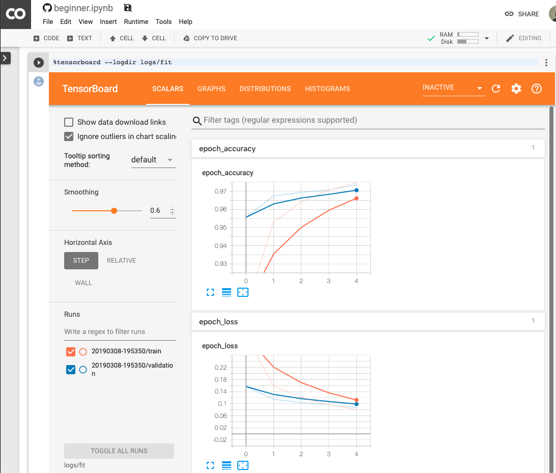
TensorBoard Imporvements
Some other features worth mention TensorBoard is now viewable directly in Jupyter Notebooks or Colab. As well their built-in data sets continue to grow.
Immediate Feedback
With TensorFlow 2.0 all code runs in eager execution, meaning every python command get executed immediately. This change improves debugging and makes it easy to convert models into graphs for easy deployment.
The team also has improved error handling, now giving you the line and file of the error so your larger projects won’t get stuck in debugging. Currently when you get an error, while you get the function in question, the actual line and filename is not provided.
Timeline to stable
As of now TensorFlow 2.0 is available in an Alpha release. They are expecting the RC to ship in spring, with the full release set for Q2 of 2019. Thanks to Google’s hard work there are converter scripts available. Google has said to be using these internally on their projects and adding to the scripts as problems come up. The converter scripts make use of the new 1.x compatibility module. This module holds some of the deprecated functions so that large applications can continue to function. The team at TensorFlow notes the converter does not update the styling to be idiomatic with 2.0 but keeps the code running in the new version.
TensorFlow Extended
For those new to TFX, this is TensorFlow’s end-to-end solution that covers you from the start of your data pipeline, all the way to serving your models and logging results. TFX is what makes TensorFlow stand out from other machine learning libraries, like PlaidML or Caffe.
Up till now, TFX was just a collection of libraries you would need to stitch together to make into a full solution. However, with the TensorFlow 2.0, the team has open sourced their large “horizontal” layers to make a complete solution available.
These new layers include:
- Shared configuration framework and Job orchestration
- Shared utilities for garbage collection, data access controls
- Pipeline storage
While all of this is exciting probably the most exciting is the Pipeline storage called Metadata store. Metadata store allows your cluster to have context between runs. Over time that allows you to have great insight on runs and experiments. You can also carry-over-state and re-use previously computed outputs to save time when retraining or making small changes.
Edge TPU
The new Edge TPU brings fast inferencing to any device. Coral has is making several products including a full dev board that I like to call the Rasberry Pie of ML. As well they have made a USB accelerator so you can easily speed up your existing boards with this new processor.
Also in the works is a small PCI-E Accelerator and System-on-Module pluggable board.
TensorFlow Light
TensorFlow Light is a stripped down runtime so that you can have on device machine learning for Android, iOS, Raspberry Pis, and now the new Edge TPU.
The only thing to note with the new version of TF Light is improved inference speeds.
| Device | Speed | Improvement |
|---|---|---|
| CPU | 124ms | Baseline |
| CPU /w Quantization | 64ms | 1.9x |
| GPU | 16ms | 7.7x (OpenGL and Metal) |
| Edge TPU | 2ms | 62x |
TensorFlow.js
The JavaScript version of TensorFlow has officially hit 1.0. This new launch includes off the shelf models for image, text, and audio.
You can now use TensorFlow.js to deploy your models to the browser, Node.js, Electron Desktop Apps, and even Mobile Native apps.
They are boasting a 9x inference speed up from last year.
Swift for TensorFlow
One of the TensorFlow projects I’m most excited about has now hit v0.2. With this release, they say Swift for TensorFlow is now ready for users to experiment with and try out, although there are still some bugs so you might want to hold off on any production releases until we get a bit further in.
fast.ai is writing a new course on Swift for TensorFlow that should be out soon to help bring you up to speed quickly on how you can be writing your ML code using Swift.
Community
TensorFlow has done a great job building its community and has a lot to update on all the things they have going on.
Getting involved
With TensorFlow ever going it can be hard to know where to jump into and contribute. They have formed new special interest groups for the community so you can take part in the area of TensorFlow you care about the most. These include:
- Networking
- TensorBoard
- Rust
- Add-ons
- IO
- Testing
- Build
Learning
To help get more people into machine learning and TensorFlow there are now two new courses to take:
- deeplearning.ai (via Coursera) Introduction to TensorFlow for AI, ML, and DL
- Udacity Intro to TensorFlow for Deep Learning
Hackathon
With TensorFlow v2.0, the team paired up with devpost to create a hackathon with $150k in prizes. Check out their page for all the details and how to submit for a chance to win.
TensorFlow World
TensorFlow is partnering with O’Reilly Media to create a week-long conference that is community focused where people all over the TensorFlow ecosystem can come together, show off, and learn from each other.
This year the conference is scheduled to take place Oct 28-31 in Santa Clara, CA. A call for papers is currently open until April 23, with a focus on real-world experiences and innovative ideas. Find more info at tensorflow.world or on twitter @TensorFlowWorld
There is still so much to talk about with all these new products and version. I highly recommend checking out TensorFlows YouTube channel for all of their session talks, as well as the new design TensorFlow site for all the goodies to be found in TensforFlow v2.0. You can get started with it today by running the following command.
pip install tensorflow==2.0.0-alpha0
The post TensorFlow Developer Summit 2019 appeared first on Big Nerd Ranch.
]]>The post macOS Machine Learning in 2019 appeared first on Big Nerd Ranch.
]]>Every company is sucking up data scientists and machine learning engineers. You usually hear that serious machine learning needs a beefy computer and a high-end Nvidia graphics card. While that might have been true a few years ago, Apple has been stepping up its machine learning game quite a bit. Let’s take a look at where machine learning is on macOS now and what we can expect soon.
2019 Started Strong
More Cores, More Memory
The new MacBook Pro’s 6 cores and 32 GB of memory make on-device machine learning faster than ever.
Depending on the problem you are trying to solve, you might not be using the GPU at all. Scikit-learn and some others only support the CPU, with no plans to add GPU support.
eGPU Support
If you are in the domain of neural networks or other tools that would benefit from GPU, macOS Mojave brought good news: It added support for external graphics cards (eGPUs).
(Well, for some. macOS only supports AMD eGPUs. This won’t let you use Nvidia’s parallel computing platform CUDA. Nvidia have stepped into the gap to try to provide eGPU macOS drivers, but they are slow to release updates for new versions of macOS, and those drivers lack Apple’s support.)
Neural Engine
2018’s iPhones and new iPad Pro run on the A12 and A12X Bionic chips, which include an 8-core Neural Engine. Apple has opened the Neural Engine to third-party developers. The Neural Engine runs Metal and Core ML code faster than ever, so on-device predictions and computer vision work better than ever. This makes on-device machine learning usable where it wouldn’t have been before.
Experience Report
I have been doing neural network training on my 2017 MacBook Pro using an external AMD Vega Frontier Edition graphics card. I have been amazed at macOS’s ability to get the most out of this card.

PlaidML
To put this to work, I relied on Intel’s PlaidML. PlaidML supports Nvidia, AMD, and Intel GPUs. In May 2018, it even added support for Metal. I have taken Keras code written to be executed on top of TensorFlow, changed Keras’s backend to be PlaidML, and, without any other changes, I was now training my network on my Vega chipset on top of Metal, instead of OpenCL.
What about Core ML?
Why didn’t I just use Core ML, an Apple framework that also uses Metal? Because Core ML cannot train models. Once you have a trained model, though, Core ML is the right tool to run them efficiently on device and with great Xcode integration.
Metal
GPU programming is not easy. CUDA makes managing stuff like migrating data from CPU memory to GPU memory and back again a bit easier. Metal plays much the same role: Based on the code you ask it to execute, Metal selects the processor best-suited for the job, whether the CPU, GPU, or, if you’re on an iOS device, the Neural Engine. Metal takes care of sending memory and work to the best processor.
Many have mixed feelings about Metal. But my experience using it for machine learning left me entirely in love with the framework. I discovered Metal inserts a bit of Apple magic into the mix.
When training a neural network, you have to pick the batch size, and your system’s VRAM limits this. The number also changes based on the data you’re processing. With CUDA and OpenCL, your training run will crash with an “out of memory” error if it turns out to be too big for your VRAM.
When I got to 99.8% of my GPU’s available 16GB of RAM, my model wasn’t crashing under Metal the way it did under OpenCL. Instead, my Python memory usage jumped from 8GB to around 11GB.
When I went over the VRAM size, Metal didn’t crash. Instead, it started using RAM.
This VRAM management is pretty amazing.
While using RAM is slower than staying in VRAM, it beats crashing, or having to spend thousands of dollars on a beefier machine.
Training on My MBP
The new MacBook Pro’s Vega GPU has only 4GB of VRAM. Metal’s ability to transparently switch to RAM makes this workable.
I have yet to have issues loading models, augmenting data, or training complex models. I have done all of these using my 2017 MacBook Pro with an eGPU.
I ran a few benchmarks in training the “Hello World” of computer vision, the MNIST dataset. The test was to do 3 epochs of training:
- TensorFlow running on the CPU took about 130 seconds an epoch: 1 hour total.
- The Radeon Pro 560 built into the computer could do one epoch in about 47 seconds: 25 minutes total.
- My AMD Vega Frontier Edition eGPU with Metal was clocking in at about 25 seconds: 10 minutes total.
You’ll find a bit more detail in the table below.
3 Epochs training run of the MNIST dataset on a simple Neural Network
| Average per Epoch | Total | Configuration |
|---|---|---|
| 130.3s | 391s | TensorFlow on Intel CPU |
| 47.6s | 143s | Metal on Radeon Pro 560 (Mac’s Built in GPU) |
| 42.0s | 126s | OpenCL on Vega Frontier Edition |
| 25.6s | 77s | Metal on Vega Frontier Edition |
| N/A | N/A | Metal on Intel Graphics HD (crashed – feature was experimental) |
Looking Forward
Thanks to Apple’s hard work, macOS Machine Learning is only going to get better. Learning speed will increase, and tools will improve.
TensorFlow on Metal
Apple announced at their WWDC 2018 State of the Union that they are working with Google to bring TensorFlow to Metal. I was initially just excited to know TensorFlow would soon be able to do GPU programming on the Mac. However, knowing what Metal is capable of, I can’t wait for the release to come out some time in Q1 of 2019. Factor in Swift for TensorFlow, and Apple are making quite the contribution to Machine Learning.
Create ML
Not all jobs require low-level tools like TensorFlow and scikit-learn. Apple released Create ML this year. It is currently limited to only a few kinds of problems, but it has made making some models for iOS so easy that, with a dataset in hand, you can have a model on your phone in no time.
Turi Create
Create ML is not Apple’s only project. Turi Create provides a bit more control than Create ML, but it still doesn’t require the in-depth knowledge of Neural Networks that TensorFlow would need. Turi Create is well-suited to many kinds of machine learning problems. It does a lot with transfer learning, which works well for smaller startups that need accurate models but lack the data needed to fine-tune a model. Version 5 added GPU support for a few of its models. They say more will support GPUs soon.
Unfortunately, my experience with Turi Create was marred by lots of bugs and poor documentation. I eventually abandonded it to build Neural Networks directly with Keras. But Turi Create continues to improve, and I’m very excited to see where it is in a few years.
Conclusion
It’s an exciting time to get started with Machine Learning on macOS. Tools are getting better all the time. You can use tools like Keras on top of PlaidML now, and TensorFlow is expected to come to Metal later this quarter (2019Q1). There are great eGPU cases on the market, and high-end AMD GPUs have flooded the used market thanks to the crypto crash.
The post macOS Machine Learning in 2019 appeared first on Big Nerd Ranch.
]]>